The model
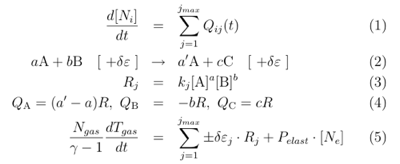 The time evolution of [Ni], density of species i = 1 … imax,is calculated using a numerical solution of the balance equations (1). Source rates Qij corresponding to different processes j = 1 … jmax are computed automatically. For example, the source rates corresponding to reaction (2) with reaction rate Rj (3), are written in (4).
The evolution of the gas temperature is determined from the solution of the heat transport equation in the form given in (5) (adiabatic isometric approximation) with known specific heat ratio. The second term in the right side corresponds to elastic election-neutral collisions and is computed using BOLSIG+ solver.
Structure
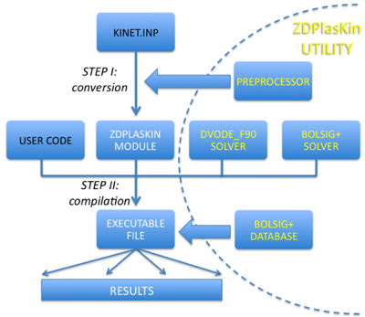 A 2-step structure was chosen to minimize computational overhead and enhance execution speed.
Step 1: The preprocessor converts the input text file into a customized Fortran module with the user-supplied chemistry incorporated directly into the code.
Step 2: The user must provide a short master code to call ZDPlasKin library routines which perform the time integration and update electron transport and rate coefficients using BOLSIG+. Output files are written and diagnostic routines are called from the master code. The master code must be compiled and linked with the ZDPlasKin fortran routines.
User requirements
The user must be able to write simple fortran code, either adapting the example master codes or starting from scratch and making calls to ZDPlasKin following the call structures defined in the user’s guide.
A typical user with some basic experience in Fortran can learn to use the basic features of ZDPlasKin in about one day. Making use of all the advanced features requires more experience and familiarity with the options available in the ZDPlasKin library routines.
A brief review of main routines
A call to the subroutine init() initializes the module and must be made before calling any of the other ZDPlasKin functions.
The main data structures are accessible from the master code, either directly as public variables and/or through function calls. For example, species densities are stored in the density(i) array, and the user can use this array in the master code to directly set (or get) values. Alternatively, the user can set (or get) values of the species densities by calling the set(get)_density(“X”,dens) subroutine. ZDPlasKin allows the user to work with species names “X” rather than a corresponding array index. If needed, the array index i of species X is available from the species_name(:) array or by calling the get_species_index( “X”,i) subroutine.
The parameters specifying the conditions of calculations can be set or accessed (get) with set(get)_conditions() routines. Required parameters are the gas temperature and the reduced electric field; optional parameters include the specific gas ratio. A logical switch is used to signal that the evolution of the gas temperature should be included in the calculation.
The principal subroutine supplied for the time integration of the rate equations is timestep(), which calls DVODE_F90, an implicit and usually very efficient and accurate integration routine. VODE is a package of subroutines for the numerical solution of the initial-value problem for systems of first-order ordinary differential equations. The package uses the fixed-leading-coefficient Backward Differentiation Formula (BDF) method for stiff systems. An alternate time integration routine is the timestep_explicit() subroutine which is an explicit, first-order accurate, Euler solver. The latter is recommended only for very specific applications (such as an integration with a small fixed timestep).
Two further routines get_density_total() and get_rates() provide output useful for analysis: the total density of all species – neutral and charged particle species – total charge density, species source terms, reaction rates and a matrix of source terms, respectively.
Subroutine write_file() writes an output list of species and reactions as well as the matrix of reaction source terms to the corresponding files.
The only configuration subroutine in the module is set_config(). It allows setting the absolute and relative errors for the DVODE solver, or it can be used to manage the silent operating mode (no screen output) and the regime of statistic acquisition.
See the user’s guide for ZDPlasKin for a detailed description of all the routines.
visualization with QTPlaskin
 We encourage users to use auto save of data in QtPlaskin-compatible format.
An adaptive auto save is triggered on calling just after initialization set_config(QTPLASKIN_SAVE=.true.). In this case, ZDPlasKin saves all necessary data in external files after every timestep. Manual data save is possible using write_qtplaskin(time) routine.
The list of saved data includes temporal dependences of key parameters (reduced electric field, gas and electron temperatures, electron current density and electric power dissipation per unit volume), density of species, reaction source rates and reaction-specific production rates of species for sensitivity analysis. User-specific data can optionally be saved.
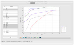
Generated in this way output can then be analyzed using QtPlaskin graphical interface developed by the TRAPPA group at the Instituto de Astrofisica de Andalucia, CSIC in Granada, Spain. Please use the following web site for downloading source or complete applications for Windows, Mac OS and Linux: http://www.trappa.es/content/software/.