These results have been presented: Pancheshnyi S., Eismann B., Hagelaar G. and Pitchford L., “ZDPLASKIN: A NEW TOOL FOR PLASMACHEMICAL SIMULATIONS”, The Eleventh International Symposium on High Pressure, Low Temperature Plasma Chemistry (HAKONE XI), September 2008, Oleron Island, France.
Here we present a 0D simulation of a high-pressure argon plasma generated in a Micro Cathode Sustained Discharged (MCSD) [1]. The MCSD is initiated between a Micro-Hollow Cathode Discharge and a third electrode that pulls the plasma outside of the micro cathode. The inter-electrode distance is of the order of a centimeter or less. We suppose that the densities are constant inside the MCSD, along the axis, and thus that the zero dimensional approximation is valid. Results from more detailed 2D calculations [2] confirm the validity of this assumption.
The behavior of argon plasmas is quite well known, even at high pressures, and this is a good example for showing the abilities of ZDPlasKin. In this particular case, we will show the possibility of coupling of homogeneous plasmachemistry with diffusion losses and a simple external circuit.
 We consider a uniform argon plasma column under the following conditions: pressures in the range of 100 torr, room temperature 300 K and small space scale 4 mm (input data required to establish the electric field and estimate the diffusion length). The results presented here were obtained for 1 kV generator voltage and 100-kOhm series resistance.
The species considered in the model are Ar, Ar* (one metastable only is taken into account, to simplify the problem), Ar+, Ar2+ and electrons. Electrons, accelerated in the electric field, collide with the neutrals to produce ionization or excitation. Those new species will disappear by recombination, collisional de-excitation (with reactions rates increasing with pressure) or diffusion (with diffusion rates decreasing with increasing pressure). After a time of the order of 1 ms for our conditions, this system reaches its stationary state where source terms for each species are exactly balanced by loss terms. The total number of processes taken into account is 12. We note, that to start a simulation, we need to put an artificial initial density of electrons to ensure the ignition of a plasma (106 cm-3 here, this could be refined to be considered more properly, for example, as the cosmic ray ionization).
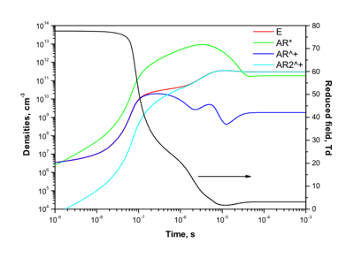
An example of species profile and reduced electric field as functions of time is presented on Figure 1.
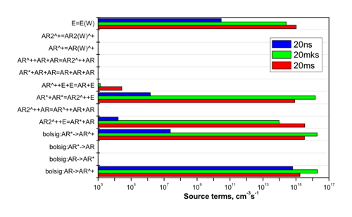 The first comments are upon the evolution of the Ar+ density: first (up to a few tens of ns), it follows the electron density while the argon metastable density is growing, triggering two-step ionization. At about 200 ns, the molecular ion Ar2+ becomes to be dominant and then the system finds its equilibrium. ZDPlasKin allows to make more precise diagnostics, as shown on Figure 2. The three bar graphs are traced at different time moments (20 ns, 20 mks and 20 ms, respectively) and represent the gain and loss terms (in absolute values) for electron density for each reaction independently.
With this tool, it is easy to see that at the very beginning, the major creation of electrons is the direct ionization, and the major loss (that obviously does not compensate the creation) is due to the diffusion. Then, at 20 mks, we still see a net creation of electrons, but the processes of gain and loss are more diverse: the losses by diffusion are dominant by a factor two over the losses by dissociative recombination and the gains are almost equally split between the direct ionization, the two-step ionization and the associative ionization. Finally, at 20 ms (a time when we can considered the plasma to be at steady state), the electron creations and losses are dominated by, on one hand, the two-step ionization, and on the other hand the dissociative recombination. From this simple case, we clearly see how convenient it is to follow any phenomenon, to identify the dominant processes, their interactions, etc …
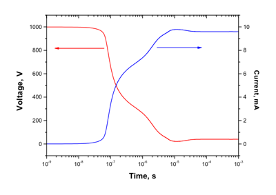 The other diagnostic concerns the gap voltage and current (Figure 3). This is the kind of output that will facilitate the comparison with experiments or with other simulations, knowing the macroscopic parameters of the problem. It also helps to trace current-voltage characteristics (storing the steady state values for various conditions of current, for example) and to see its evolution as the pressure is changing, for example. On this graph, we see the drop in the voltage that indicates the beginning of the discharge, and the corresponding increasing current due to the electron avalanche. This output can also be a way of estimating the breakdown voltage of a plasma in given conditions: if the voltage does not drop for a certain value, and, when it is increased a bit, it does, then we have the signature of a breakdown and thus the corresponding voltage.
[1] R.H. Stark and K.H. Schoenbach, J. Appl. Phys. 85 2075 (1999).
[2] K. Makasheva, E Munoz-Serrano, G. Hagelaar, J.P. Boeuf and L.C. Pitchford, Plasma Phys. Control. Fusion 49 B233 (2007).
Required files
The input text file kinet.inp can be written using any editor. This input file is converted to a Fortran module using the PREPROCESSOR utility provided in the download package. An example of the Fortran code corresponding to above-mentioned kinet.inp file is zdplaskin_m.F90. The generated Fortran code is intended to be used as a “black box”.
Required cross sections for electron processes with species indicated in section BOLSIG have to be stored in bolsigdb.dat data file. In the present example, these electron cross sections were retrieved from ELECTRON SCATTERING DATABASE, SIGLO database. Note, ionization from the metastable state Ar* is taken into account in the list of processes while this process is not in the list of processes supplied in the download file. User must extend it adding the corresponding cross-section; we show here an example of these data at the end of bolsigdb.dat file.
User code here consists of two files: the principal code master_code.F90 and a module master_module.F90. These files must be compiled, using a Fortran 90/95 compiler, along with DVODE solver and ZDPLASKIN module in the following order: dvode_f90_m.F90 – master_module.F90 – zdplaskin_m.F90 – master_code.F90, and linked with the BOLSIG+ binary library (bolsig.xxx). External parameters (gas temperatures and pressure, dimensions of plasma channel, voltage and serial resistance, initial electron density and the time of calculation) are red from the external file conditions.ini. Typical screen output is in out.txt.
You can download all these files in a zip archive.
 This test case corresponds to a nitrogen plasma consisting of electrons, N2, N2(A), N2(B), N2(a’), N2(C), N, N+, N2+, N3+, N4+ and includes 36 processes. The BOLSIG+ solver is evoked to calculate the rates of excitation and ionization by electron impact. The reaction rates for heavy species are mostly taken from [1]. An effective ion-neutral collision temperature is calculated in this case using known electric field, mobilities and masses of species as it is proposed in [1].
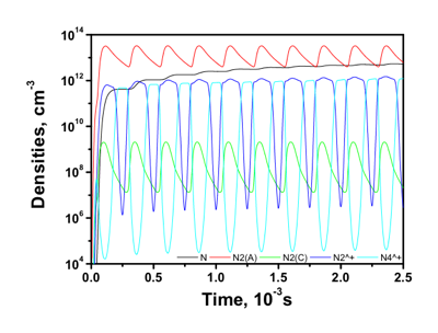 Corresponding lines are placed at the beginning of REACTION section in input text file kinet.inp. This input file is converted to a Fortran module using the PREPROCESSOR utility provided in the download package. An example of the Fortran code corresponding to above-mentioned kinet.inp file is zdplaskin_m.F90.
 This test case corresponds to an Ar plasma consisting of electrons, atomic ions, and neutrals. The charged particles are supposed to be generated by direct electron impact ionization and lost by 3-body recombination: